High Energy Astronomy News

Two items of note:

1. Scientific American has a nice article on why the threat to life on Earth from Gamma Ray Bursts, in particular from the dying start Eta Carinae, is not something you need to worry about. (I've discussed putative GRB-caused events here and here).
2. NuSTAR, an orbitting hard X-ry telescope, has captured some cool images of hard X-ray emission from the Sun (not a target NuSTAR was expected to look at, being designed for the study of Active Galactic Nuclei millions to billions of light years from Earth).

The NuSTAR data, seen in green and blue, reveal solar high-energy emission (green shows energies between 2 and 3 kiloelectron volts, and blue shows energies between 3 and 5 kiloelectron volts). The high-energy X-rays come from gas heated to above 3 million degrees. The red channel represents ultraviolet light captured by SDO at wavelengths of 171 angstroms, and shows the presence of lower-temperature material in the solar atmosphere at 1 million degrees. [Image and caption from NASA/JPL]

Hooray, Octave supports numpy-style boolean array indexing operations

I've only just discovered that Gnu Octave (the Gnu version of Matlab) supports numpy-style boolean array indexing operations, in particular

• logical operations on vectors to return boolean true/false vectors
• array indexing using vectors on vectors

An example, using a simple vector a.

octave:2> a=[1 2 3 4 1 2 3 4]
a =

   1   2   3   4   1   2   3   4

Create a boolean mask called b with all elements of a greater than 2.

octave:3> b=a > 2
b =

   0   0   1   1   0   0   1   1

Now use b to access only those elements of a that are true in the mask array b.

octave:4> a(b)
ans =

   3   4   3   4

Why use Octave when we have python/numpy/scipy? Sometimes its just faster to fire up octave to get a look at data, and matlab/octave syntax is much less verbose than python.

More on the possible AD 774/775 hit on the Earth by a nearby GRB

I hadn't heard of either the odd AD 774/775 values of the C12/C14 and increased B10 ratios or the hypothesized casue: a nearby (within the Milky Way) Gamma Ray Burst before reading a blog post by Greg Laden related to climate change a while ago.

It turns out the GRB hypothesis was only recently advanced: Hambaryan & Neuhäuser, 2013, MNRAS, 430, 32 [full article text available online here]. Back at the time Phil Plait actually covered the story in his blog, which has a nice write up of the idea and why other explanations (Solar Flare, Magnetar, nearby Supernova) are claimed to be less likely than a "short" (neutron-star merger induced) GRB.

It somewhat surprises me that an event of the magnitude necessary to alter the isotopic composition of the Earth's atmosphere in less than a few seconds could occur without (a) anyone seeing anything and recording it, and more over (b) not causing any significant biological events (e.g. animal, plant or human deaths). Still, reality often runs counter to naive expectation (i.e. "common sense") so I'm not too put off the idea by that.

For now I'd view this idea of the Earth getting hit by a short GRB as a plausible hypothesis rather than concrete fact, at least until several more studies come to the same conclusion. Still, it is a rather fun and exciting idea.

What happened in the year 774/775?

Something odd happened to the Earth around the year 774/775. For the background, head over to Gred Laden's blog, where this is just part of a larger question about climate reconstruction.

A few exerts follow to give you  a taste of what caught me eye.

A long time ago, probably in our galaxy but kind of far away, a cosmic event happened that caused the Earth to be bathed in Gamma rays in AD 774 or 775.
...
There is chemical and physical evidence, though, of the Gamma ray burst. The best evidence is the large scale conversion of stable Nitrogen isotopes into unstable Carbon–14 isotopes in the upper atmosphere. As you know, radioactive (meaning, unstable) Carbon–14 is created continuously but at a somewhat variable rate in the upper atmosphere. Some of that Carbon is incorporated, along with regular stable Carbon, into living tissues. After the living tissue is created and further biological activity that might retrofit some of the Carbon atoms ends (i.e., the thing dies) the ratio of radioactive Carbon to stable Carbon slowly changes as the radioactive Carbon changes back into Nitrogen. By measuring the ratio now, we can estimate how many years ago, plus or minus, the originally living thing lived and died. But it does vary. Solar activity, nuclear testing, other things, can change the amount of Carbon–14 that gets produced. And, a cosmic event that happened in 774/775 caused the production of enough Carbon–14 to throw off the chronology by hundreds of years.

Now why haven't I heard of this event before? How certain are we that it was a Gamma Ray Burst, and if so, where was the source?

Fifteen years in orbit and awesome: The Chandra X-ray Observatory

Yesterday, July 25rd, 2014, marked the 15th anniversary of the launch of one of NASA's Great Observatories: the Chandra X-ray Observatory. I was one year into my first post-doc at Johns Hopkins at the time, and watched the launch in one of the conference rooms on the 1st floor. Later I spent many years working on data from Chandra. I can't believe its been so long.

Over-views of the 15 years of Chandra:

• "Chandra Has Been X-Raying the Universe for 15 Years" on io9.
• NASA's Chandra X-ray Observatory Celebrates 15th Anniversary at NASA.gov.
• NASA's Chandra X-ray Observatory Celebrates 15th Anniversary at the Chandra X-ray Observatory website. 

For information on the accompanying press release image go here.

An introduction to quantitative astrophotography on Linux: Part 2 - RAW to FITS and Dark Frames

In part 1 of this series I introduced my reasons for wanting to look into what I called quantitative astrophotography, by which I mean getting god quantitative estimates of the performance of a very simple, entry level, set of DSLR images of the night sky. I wanted to control and understand the quantitative changes made to the images, and hence chose to avoid the Windows-based GUI software common in the amateur astronomy world. Instead I'll use standard astronomical data reduction and analysis techniques and stick to open source tools running under Linux (actually in this case, OSX with macports).

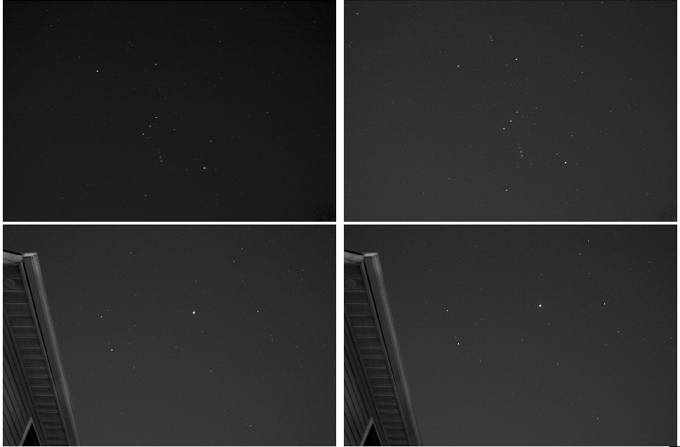
By the end of part 1 I was in possession of ~30 RAW images taken with a Canon Digital Rebel XTi, including a series of dark frames and bias frames. This article covers the next step in the process: converting the RAW images into FITS format, along with a quick look at the dark frame properties. The process of finding the bad pixels and removing them from the images will be covered in Part 3.

The flow chart summarizes the actions that need to be performed on the RAW images to end up with FITS images that have had the bad pixels, the dark current and the bias removed.

The basic idea behind astronomical imaging is to use a series of calibration images to improve the final image of the target. At these early stages of reduction we're talking about using dark frames, bias frames, and bad pixel masks to remove the additional signal in the image that is not from the sky, but from the detector electronics itself. Originally I wrote a lengthy description of each of these calibration image types, but I know think it is better just to point interested readers at more extensive discussions at:

1. Starizona's Guide to CCD Imaging.
2. Mischa's Data Reduction web page at the University of Bonn.

The other reason I decided to cut down on the terminology discussion is that is very CCD-centric, as they are the classic detector type used in professional astronomy. However digital cameras almost always use CMOS detectors and not classic CCDs. The on-Camera data processors inside digital camera perform operations that alter the data values in ways that professional CCD imagers do not.

dcraw to FITS.

To create a FITS file from a RAW file we use the -c flag on the dcraw command line and pipe the output into a program that can convert PNM format to FITS. The dcraw web page recommends pnmtofits, e.g.

dcraw -c (other_flags) input_image.cr2 | pnmtofits > output.fits

However there is one problem with this. dcraw and many image processing utilties assume the first pixel is the top left of an image, whereas the FITS conventsion is the first pixel is the bottom left. So FITS files created with pnmtofits are upside-down. ImageMagick is smart enough to know about fits and corrects for this, so we can make correctly-oriented FITS files like this:

dcraw -c (other_flags) input_image.cr2 | convert pnm:- output.fits

Dark and/or Bias Frame Creation

The dark and bias frames are not exposed to light, so the Bayer RGB mask on top of the detector is not important and the signal doesn't depend on whether each pixel is R, G or B. This means we convert the RAW file to a single channel (grayscale) image for analysis.

It is important that both the raw count output from the camera's ADU and image orientation are preserved, i.e. no gamma correction or histogram manipulation should be performed on the raw file. We want the exact 12-bit (or 14-bit if you have a newer camera) values [except that we cannot control what the Camera's image processor does to the RAW images].

The corresponding dcraw command line options are -D -4 -j -t 0. Hence for each raw format dark and/or bias frame we initially run the following command to convert to FITS:

dcraw -c -D -4 -j -t 0 input_dark.cr2 | convert pnm:- output_dark.fits

Dark and Bias Frame Statistics

The following table summarizes some simple statistical properties of all the dark and bias frames I took. The file name also contains the ISO value (400, 800 or 1600) and whether bad pixel had been removed in the dcraw to FITS conversion, where "nobadpix" means "no bad pixel removal". We'll deal with the bad pixel identification and removal in the next post.

File	Rows	Cols	Mean +/- StdDev	Median	Minimum	Maximum
Prior to bad pixel removal
dark_0694_t30.0_800_Sat_Jan_18_22:04:46_2014_nobadpix.fits	2602	3906	256.11 +/- 6.39	256.50	170.5	4056.5
dark_0695_t30.0_800_Sat_Jan_18_22:05:41_2014_nobadpix.fits	2602	3906	256.11 +/- 6.34	256.50	177.5	4056.5
dark_0696_t30.0_1600_Sat_Jan_18_22:06:22_2014_nobadpix.fits	2602	3906	256.42 +/- 10.89	257.50	95.5	4057.5
dark_0697_t30.0_1600_Sat_Jan_18_22:06:57_2014_nobadpix.fits	2602	3906	256.38 +/- 10.84	257.50	105.5	4057.5
dark_0698_t30.0_400_Sat_Jan_18_22:07:40_2014_nobadpix.fits	2602	3906	255.99 +/- 4.03	255.50	219.5	4055.5
dark_0699_t30.0_400_Sat_Jan_18_22:08:14_2014_nobadpix.fits	2602	3906	256.00 +/- 4.02	255.50	218.5	4055.5
bias_0700_t0.00025_400_Sat_Jan_18_22:09:03_2014_nobadpix.fits	2602	3906	255.99 +/- 2.95	255.50	210.5	333.5
bias_0701_t0.00025_400_Sat_Jan_18_22:09:09_2014_nobadpix.fits	2602	3906	256.00 +/- 2.94	255.50	216.5	328.5
bias_0702_t0.00025_800_Sat_Jan_18_22:09:21_2014_nobadpix.fits	2602	3906	256.09 +/- 4.98	256.50	175.5	397.5
bias_0703_t0.00025_800_Sat_Jan_18_22:09:23_2014_nobadpix.fits	2602	3906	256.09 +/- 4.98	256.50	185.5	394.5
bias_0704_t0.00025_1600_Sat_Jan_18_22:09:31_2014_nobadpix.fits	2602	3906	256.39 +/- 9.27	257.50	101.5	531.5
bias_0705_t0.00025_1600_Sat_Jan_18_22:09:32_2014_nobadpix.fits	2602	3906	256.39 +/- 9.27	257.50	99.5	534.5
Bad pixels removed
dark_0694_t30.0_800_Sat_Jan_18_22:04:46_2014.fits	2602	3906	256.10 +/- 5.04	256.50	193.5	320.5
dark_0695_t30.0_800_Sat_Jan_18_22:05:41_2014.fits	2602	3906	256.10 +/- 5.04	256.50	177.5	693.5
dark_0696_t30.0_1600_Sat_Jan_18_22:06:22_2014.fits	2602	3906	256.40 +/- 9.41	257.50	95.5	1047.5
dark_0697_t30.0_1600_Sat_Jan_18_22:06:57_2014.fits	2602	3906	256.36 +/- 9.39	257.50	105.5	670.5
dark_0698_t30.0_400_Sat_Jan_18_22:07:40_2014.fits	2602	3906	255.99 +/- 2.96	255.50	219.5	451.5
dark_0699_t30.0_400_Sat_Jan_18_22:08:14_2014.fits	2602	3906	255.99 +/- 2.95	255.50	218.5	316.5
bias_0700_t0.00025_400_Sat_Jan_18_22:09:03_2014.fits	2602	3906	255.99 +/- 2.95	255.50	210.5	307.5
bias_0701_t0.00025_400_Sat_Jan_18_22:09:09_2014.fits	2602	3906	256.00 +/- 2.94	255.50	216.5	299.5
bias_0702_t0.00025_800_Sat_Jan_18_22:09:21_2014.fits	2602	3906	256.09 +/- 4.98	256.50	175.5	341.5
bias_0703_t0.00025_800_Sat_Jan_18_22:09:23_2014.fits	2602	3906	256.09 +/- 4.98	256.50	185.5	340.5
bias_0704_t0.00025_1600_Sat_Jan_18_22:09:31_2014.fits	2602	3906	256.39 +/- 9.27	257.50	101.5	418.5
bias_0705_t0.00025_1600_Sat_Jan_18_22:09:32_2014.fits	2602	3906	256.39 +/- 9.27	257.50	102.5	434.5

We can immediately see that the RAW values have been altered by the on-camera image processing chip.

1.  The mean and median values of all the dark frame and bias frames are essentially 256+/-1, irrespective of whether it is a 30 second dark frame or a 1/4000'th of a second bias exposure, and irrespective of the ISO value or whether bad pixels have been removed. That value of 256 is 2^8, which would be highly suggestive of a camera-processor induced value even if we didn't already suspect some on-board processing of the RAW frames.
2. The standard deviations of the mean don't relate the mean values. 

In the next post in this series we will look at bad pixel detection and removal using dcraw.

How much does a square root cost?

An interesting diversion: how much (time) does calling the square root function sqrt() cost, and is it even worth trying alternative less-accurate implementations?

Some Assembly Required provides some answers: 

SQUARE ROOT

Method	Total time	Time per float	Avg Error
Compiler sqrt(x) / x87 FPU FSQRT	404.029ms	24ns	0.0000%
SSE intrinsic ssqrts	200.395ms	11.9ns	0.0000%
Carmack’s Magic Number rsqrt * x	72.682ms	4.33ns	0.0990%
SSE rsqrtss * x	20.495ms	1.22ns	0.0094%
SSE rsqrtss * x with one NR step	53.401ms	3.18ns	0.0000%
SSE rsqrtss * x with one NR step, unrolled by four	48.701ms	2.90ns	0.0000%

RECIPROCAL SQRT

Method	Total time	Time per float	Avg Error
Carmack’s Magic Number rsqrt	59.378ms	3.54ns	0.0990%
SSE rsqrtss	14.202ms	0.85ns	0.0094%
SSE rsqrtss with one NR step	45.952ms	2.74ns	0.0000%

Useful OSX-specific command line tools

Life-hacker has a short list of uses OS X command line programs that aren't just standard GNU/*nix commands: http://lifehacker.com/eight-terminal-utilities-every-os-x-command-line-user-s-1593793109

This mentions homebrew, which I hadn't heard of before. This answer to a stack overflow question about what are the differences between homebrew and macports gives some info (install location, user space vs sudo use, number of packages, support for multiple versions etc) but may not be enough to allow a definite decision on which to use without some experimentation. For science it appears currently homebrew has some but not all of the standard packages I'd expect.

The (Forever) Language War

I generally find comparisons between programming languages to be a waste of time given they're largely based on personal preference over objective metrics, and even metric-based comparisons are often superficial or downright misleading (yeah, I'm talking about you Julia). Generally my view is use what best fits the application modulo your expertise, and the language doesn't really matter - it is an implementation choice.

That said, I've lately being feeling rather down about C++ which is the language I develop in most heavily. Sure, it has speed and expressive power but some of the most powerful features are semantically non-trivial and most galling of all, it really doesn't come with many standard "packages" in the way Java and Python do. OK, it comes with the STL, which I do like, but then you have to go to Boost, and then you look at how some of the Boost packages are coded and you wonder if it is even the same language. In a very large and complicated project I find the developer (or more technically, integration troubleshooter and debugger) role to have low productivity. It isn't as bad as perl but it is easy for "other" programmers to write code that is just overly complicated for the job. Oh great, someone has learnt about the Abstract Factory pattern, and has decided to use it everywhere: attempt to drill down through layers of unnecessary obfuscatory abstraction (that manages to be coupled to a million other things instead of decoupling the way abstraction should do) to find what some code is actually doing. Analyze, debug, code, compile ... ... ... and run again, all while you have a supposedly critical release deadline looming.

It is easy to forget the problem what C++ set out to fix, which I was reminded of when I starting reading "Learning OpenCV". Now OpenCV is a wonderfully powerful open source library in my opinion, based on mainly using it before now through its Python bindings. But reading how to use the C API was eye opening. What, I have to remember to delete those resources? Oh great, void* pointers and I have to remember what type to cast to/from. I could just imagine the fun bugs someone had to deal with. Suddenly C++ didn't seem so doddering.

While reading about Apple's new Swift language at Slate.com (Another new proprietary language to tie developers to Apple and in darkness bind them, how exciting for the Mac fan boys!) I came across a link to a discussion by David Green comparing his experience trying out both iOS and Android development tools. The comments are the article reveal the pattern that makes me dislike language comparisons: In a discussion of X and Y you must be biased toward X because you know more about it X so really X and Y are equally good. (There should be a name for this fallacy but I can't seem to find it). However the article itself is worth a look, because it compares the iOS+Xcode+Objective-C platform to Android+Eclipse+Java platform in terms of ease of development. I've always been somewhat curious about Xcode and Objective-C, but David Green's article is enough to stop me wasting my time. What the commentators on his article don't understand is that while you can do great stuff with Xcode and Objective-C it has placed extra hurdles in your way: the extra verbosity needed in the language, the extra time it'll take to hunt down solutions to non-trivial problems. That time might not matter to some developers, in particular to Apple-only developers, but it will to matter to someone and it certainly matters to me.

Plotting images with axis coordinates in Octave

It is remarkable that I've struggled to find any examples in the Octave documentation or other people's tutorials or examples on how to plot an image (or matrix) with axis coordinates that aren't the pixel or cell numbers.

function image_with_axes()
    clear all;
    more off;
   
    % These are our eventual axis coordinates.
    x = linspace(-10,10,100);
    y = x - 2;
   
    % Generate an Airy disk
    [xg,yg]=meshgrid(x,y);
    rad = sqrt( xg.^2 + yg.^2);
    airy = besselj(1,rad)./rad;
    airyintensity = abs(airy).^2;
   
    % The normal imagesc invocation. Note axis ratio.
    figure(1);
    imagesc(airyintensity)
    axis image
    %colorbar
   
    % Now invoke with axis vectors before the image/matrix
    figure(2);
    imagesc(x,y,airyintensity);
    axis image
    %colorbar
   
    % Demonstrate the coordinates a little more clearly
    % Coordinate axes are taken to be the center of the
    % image pixel.
    a=rand(4);
    x=[3:6];
    y=[-1:2];
    figure(3);
    imagesc(x,y,a);
   
    % What about non-linear axes. Not handled correctly like this.
    % This case is dealt with another time,
    figure(4);
    x2=sqrt(x)
    y2=x.^2
    imagesc(x2,y2,a);

endfunction

SN 2014J update

I've been exceptionally busy lately, and haven't had any time to follow up on what observations of SN 2014J have told us. A google search didn't show very much, so I ended up searching Arxiv.org for papers associated with SN 2014J returns the following list (search http://arxiv.org/find/all/1/all:+2014J/0/1/0/all/0/1):

1. arXiv:1405.1488 [pdf, other]

No X-rays from the very nearby Type Ia SN2014J: constraints on its environment

R. Margutti, J. Parrent, A. Kamble, A.M. Soderberg, R.J. Foley, D. Milisavljevic, M.R. Drout, R. Kirshner

Comments: 9 pages, Submitted to ApJ

2. arXiv:1404.2639 [pdf, ps, other]

Diffuse Interstellar Bands vs. Known Atomic and Molecular Species in the Interstellar Medium of M82 toward SN 2014J

Daniel E. Welty (1), Adam M. Ritchey (2), Julie A. Dahlstrom (3), Donald G. York (1) ((1) Univ. of Chicago, (2) Univ. of Washington, (3) Carthage College)

Comments: 27 pages, 6 figures, submitted to ApJ (comments welcome)

3. arXiv:1403.7405 [pdf, ps, other]

Supernova 2014J at maximum light

D.Yu.Tsvetkov, V.G. Metlov, S.Yu. Shugarov, T.N. Tarasova, N.N. Pavlyuk

Comments: 10 pages, 4 figures, submitted to Contrib. Astron. Obs. Skalnate Pleso

4. arXiv:1403.4250 [pdf, other]

Constraints on the Progenitor System of the Type Ia Supernova 2014J from Pre-Explosion Hubble Space Telescope Imaging

Patrick L. Kelly, Ori D. Fox, Alexei V. Filippenko, S. Bradley Cenko, Lisa Prato, Gail Schaefer, Ken J. Shen, WeiKang Zheng, Melissa L. Graham, Brad E. Tucker

Comments: Submitted to ApJ, comments welcome

5. arXiv:1402.4806 [pdf, ps, other]

Expectations for the Hard X-ray Continuum and Gamma-ray Line Fluxes from the Type Ia supernova SN 2014J in M82

Lih-Sin The, Adam Burrows

Comments: Accepted to the Astrophysical Journal (March 31, 2014), with one additional figure and further discussion of technique

6. arXiv:1402.2717 [pdf, ps, other]

Specific predictions for SN 2014J in the context of the Quark Nova Ia model

Rachid Ouyed (1), Nico Koning (1), Denis Leahy (1), Jan E. Staff (2) ((1) Department of Physics and Astronomy, University of Calgary, Calgary, Alberta, Canada, (2) Department of Physics and Astronomy, Macquarie University, Australia)

Comments: 3 pages

7. arXiv:1401.7968 [pdf, ps, other]

Estimating the First-Light Time of the Type Ia Supernova 2014J in M82

WeiKang Zheng, Isaac Shivvers, Alexei V. Filippenko, Koichi Itagaki, Kelsey I. Clubb, Ori D. Fox, Melissa L. Graham, Patrick L. Kelly, Jon C. Mauerhan

Comments: Accepted for publication in ApJ Letters

This is quite a varied set of papers. I quite like the Margutti et al paper, not just because it is on X-ray emission but because of the impressive figures.

Otherwise, the most interesting of the bunch is Zheng et al. Not only did they uncover some earlier but unrecognized observations of the supernova, but the managed to estimate the explosion time (*) at Jan 14.75 UT (2014), about a week before Fossey's UCL undergraduates first noticed it. Tsvetkov et al present UVBRI light and color curves and conclude that SN 2014J belongs the the "normal" [Quotation marks in the original] subset of Type 1a SNe. How this matches up with the unusual early-time powerl-law light curve Zheng discovered doesn't seem to be discussed in their article, and as the subject is out of my (former) expertise I don't have enough information to make an informed speculation.

(*) Technically the time that any light from the explosion would have passed Earth. At a distance of D~3.5 Megaparsecs the actual explosion occurred ~11 million years ago (i.e. well before our ancestors and the ancestors of chimpanzees split off from each other).

Supernova 2014J in M82: Some more pictures and how to spot it

The Type Ia supernova 2004J in M82 is near peak brightness, and should be easy to spot if you live in the northern hemisphere and have a small telescope or large binoculars. Brian Dodson has a good guide to finding it on the sky.

Here are two more images of M82 taken by Swift UVOT, the second taken some years before the SN and the first taken on January 22, the day after its initial discovery. [Images from NASA/GSFC media site, credit NASA/Swift/P. Brown, TAMU]. Note that the SN is circled in the first image. The large white blob surrounding a blue and white point is not the SN, but a bright foreground star.

An introduction to quantative astrophotography on Linux: Part 1

My work duties briefly had me thinking about some basic astronomical image processing questions that ultimately did not need to be solved as part of that project. Nevertheless the issue was interesting enough to make me perform a simple astrophotography experiment with a normal camera and some open-source software. As many of the astro-photography websites I browsed as part of my research for the work project, and for this experiment, used much expensive hardware and essentially “black-box” GUI Windows-based software, I thought it would be possibly helpful to publish my experiences on this blog.

The aims

The aims of this first experiment are to get answers to the following questions:

1. What kind of astrophotography can be accomplished with a basic DSLR and a static tripod in the middle of suburbia? What kind of spatial resolution, signal-to-noise, and limiting magnitude can we achieve without specialized equipment?
2. What are the basic physical characteristics of DSLR astronomical imagery? How big are the pixel sizes, what are the dark current and bias levels, etc etc?
3. Can satellites, in particular Geostationary satellites, be imaged with such a simple set of equipment? They definitely can be with slightly better equipment - see Dave Kodama’s astrophotography page and Sinnbilder’s post at DPReview.
4. How easy is it to process RAW files into a format that quantitative astrometry and photometry can be performed on them, using only open source software?

The equipment

• A Canon Digital Rebel XTi (aka EOS 400D) using the standard “kit” 18-55mm f/3.5-5.6 lens.
• A nice lightweight tripod who make and model I cannot remember.
• A computer (a 2008-era Aluminum body 13” Macbook running OS X 10.8 and more importantly using macports for the open-source software). Processing (see later articles) would have been easier if I’d used Linux directly but it was simply more convenient for me to use this old Macbook’s OS directly without resorting to the use of a desktop or a virtual Linux machine.

The observations

On a cold January night (22 degrees Fahrenheit) that was apparently cloudless I set the camera to shoot in RAW mode with 30 second exposures. This is is suburbia, so the site was not totally free of light pollution from the various deck-lights and streetlights associated with the surrounding houses. I had trouble getting the lens in focus by hand, so back inside I set the lens to AF and camera to auto everything and focussed on the most distant thing I could across the house.

I set the tripod and camera up on our deck and started by taking a series of 30 second images of Orion. I chose Orion as the excellent Satellite AR app on my android phone showed an arc of Geostationary satellites going through the southern half of Orion. I experimented with different ISO levels during the run, 400, 800 and 1600 as I was interested in noise levels and star brightness as a function of ISO, and also was worried about saturation of the brighter stars. In future I will use ISO 1600 throughout the night.

Following the Orion images I took a series of images of the field around Jupiter, which was quite bright that night and up in Gemini. I was wondering if  the planet’s image would be resolved, whether could the moons be separated from the planet, and whether the apparent motion of the planet across of the sky could be distinguished from the sidereal motion of the stars.

Finally I took a set of 30 second dark frames: two exposures each as each ISO, and them two 1/4000 second exposures at each ISO. The later images will be used to determine bias levels. I was careful to make sure these images were taken while outside at the same temperature as the observations, as the dark current can be expected to be temperature dependent.

I forgot to take any “dome” flats when I went inside, and finding something white and uniformly illuminated in the house was so difficult that I gave up on getting any rough flats for this first experiment.

FileName     DateTime                  ISO   tsec fstop flen rows cols target _MG_0670.CR2 Sat_Jan_18_21:47:25_2014  400     30 f/5.6 30.0 2602 3906 orion _MG_0671.CR2 Sat_Jan_18_21:48:17_2014  400     30 f/5.6 30.0 2602 3906 orion _MG_0672.CR2 Sat_Jan_18_21:48:57_2014  400     30 f/5.6 30.0 2602 3906 orion _MG_0673.CR2 Sat_Jan_18_21:49:37_2014  400     30 f/5.6 30.0 2602 3906 orion _MG_0674.CR2 Sat_Jan_18_21:51:05_2014  800     30 f/5.6 30.0 2602 3906 orion _MG_0675.CR2 Sat_Jan_18_21:51:45_2014  800     30 f/5.6 30.0 2602 3906 orion _MG_0676.CR2 Sat_Jan_18_21:52:25_2014  800     30 f/5.6 30.0 2602 3906 orion _MG_0677.CR2 Sat_Jan_18_21:53:05_2014 1600     30 f/5.6 30.0 2602 3906 orion _MG_0678.CR2 Sat_Jan_18_21:53:55_2014 1600     30 f/5.6 30.0 2602 3906 orion _MG_0679.CR2 Sat_Jan_18_21:54:34_2014 1600     30 f/5.6 30.0 2602 3906 orion _MG_0680.CR2 Sat_Jan_18_21:55:23_2014 1600     30 f/5.6 30.0 2602 3906 orion _MG_0681.CR2 Sat_Jan_18_21:56:07_2014  800     30 f/5.6 30.0 2602 3906 orion _MG_0682.CR2 Sat_Jan_18_21:56:42_2014  800     30 f/5.6 30.0 2602 3906 orion _MG_0683.CR2 Sat_Jan_18_21:57:19_2014  800     30 f/5.6 30.0 2602 3906 orion _MG_0684.CR2 Sat_Jan_18_21:57:55_2014  800     30 f/5.6 30.0 2602 3906 orion _MG_0685.CR2 Sat_Jan_18_21:59:11_2014  800     30 f/5.6 30.0 2602 3906 jupiter _MG_0686.CR2 Sat_Jan_18_21:59:49_2014  800     30 f/5.6 30.0 2602 3906 jupiter _MG_0687.CR2 Sat_Jan_18_22:00:27_2014  800     30 f/5.6 30.0 2602 3906 jupiter _MG_0688.CR2 Sat_Jan_18_22:01:03_2014  800     30 f/5.6 30.0 2602 3906 jupiter _MG_0689.CR2 Sat_Jan_18_22:01:38_2014  800     30 f/5.6 30.0 2602 3906 jupiter _MG_0690.CR2 Sat_Jan_18_22:02:13_2014  800     30 f/5.6 30.0 2602 3906 jupiter _MG_0691.CR2 Sat_Jan_18_22:02:49_2014  800     30 f/5.6 30.0 2602 3906 jupiter _MG_0692.CR2 Sat_Jan_18_22:03:26_2014  800     30 f/5.6 30.0 2602 3906 jupiter _MG_0693.CR2 Sat_Jan_18_22:04:02_2014  800     30 f/5.6 30.0 2602 3906 jupiter _MG_0694.CR2 Sat_Jan_18_22:04:46_2014  800     30 f/5.6 30.0 2602 3906 dark _MG_0695.CR2 Sat_Jan_18_22:05:41_2014  800     30 f/5.6 30.0 2602 3906 dark _MG_0696.CR2 Sat_Jan_18_22:06:22_2014 1600     30 f/5.6 30.0 2602 3906 dark _MG_0697.CR2 Sat_Jan_18_22:06:57_2014 1600     30 f/5.6 30.0 2602 3906 dark _MG_0698.CR2 Sat_Jan_18_22:07:40_2014  400     30 f/5.6 30.0 2602 3906 dark _MG_0699.CR2 Sat_Jan_18_22:08:14_2014  400     30 f/5.6 30.0 2602 3906 dark _MG_0700.CR2 Sat_Jan_18_22:09:03_2014  400 1/4000 f/5.6 30.0 2602 3906 bias _MG_0701.CR2 Sat_Jan_18_22:09:09_2014  400 1/4000 f/5.6 30.0 2602 3906 bias _MG_0702.CR2 Sat_Jan_18_22:09:21_2014  800 1/4000 f/5.6 30.0 2602 3906 bias _MG_0703.CR2 Sat_Jan_18_22:09:23_2014  800 1/4000 f/5.6 30.0 2602 3906 bias _MG_0704.CR2 Sat_Jan_18_22:09:31_2014 1600 1/4000 f/5.6 30.0 2602 3906 bias _MG_0705.CR2 Sat_Jan_18_22:09:32_2014 1600 1/4000 f/5.6 30.0 2602 3906 bias

Initial Outcome

Two of Orion and two of the Jupiter/Gemini images, after bad-pixel and dark current removal, lightly smoothed and on a Log10 intensity scale.

Going through the images on the camera showed I’d had a good series of Orion images, with the sword being very prominent compared to the view “by eye”. The motion of the stars was clearly apparent even within the 30 s exposures, and over the entire series the stars moved many degrees. In contrast a Geostationary satellite would be at the exact same location in each image. Some (processed) frames are shown.

The Jupiter/Gemini images were also of reasonable quality. The dark frames (discussed in a future post) clearly showed a number of bad pixels in the camera that are not normally apparent in well-lit normal exposures.

Next episode...

In the next part of this series (Part 2) I’ll cover the steps of converting the RAW files on the camera into the FITS format used by professional astronomers and professional astronomical software.

New supernova in M82!

Students at UCL have discovered a new Supernova in M82. This is the first optically visible SN in M82 since I can't remember when, and its location is a kpc or two out from the nucleus (where there is an optically-obscured core-collapse Supernova every 10-20 years or so) seems consistent with the preliminary reports of it being a SN type Ia.

This image is from the UCL press release:  http://www.ucl.ac.uk/maps-faculty/maps-news-publication/maps1405. The first image was taken in December 2013, the second on January 21st 2014.

Digital Camera detector sizes and noise characteristics

The following sites contain some useful information regarding the physical sizes of certain digital camera CCDs, pixel sizes in microns, and noise characteristics and gains at different ISO levels.

• Roger Clark's compilation of gain, readout noise, detector and pixel sizes for a variety of digital cameras.
• Gain, readout noise in ADU and electrons, pixel sizes etc for EOS 10D and EOS 20D. Includes a nice set of examples astro-photography images and dark frames.

Why is this important? Its related to a project I'm working on at the moment. This kind of information is very difficult to find on manufacturer's sites, as they're catering to an audience who has been make to think that number of megapixels is the only metric of value.

Other useful links:

• dcraw: Read and convert RAW files (of all the various types).
• rawtran: A wrapper around dcraw to support better conversion of RAw to FITS than the cruder method suggested by dcraw. This is related to the munipack software package.

Molten iron storm clouds

Here is some pretty cool research on Brown Dwarfs (or Dwarves?) using the Spitzer Space Telescope. Researchers expected that Brown Dwarfs should show variations in brightness due to storms in their atmospheres, which are more like extreme versions of giant planets like Jupiter than the atmospheres of actual stars like the Sun. When they went looking with the SST they found even more variation in brightness than expected.

The really cool part: the clouds aren't made of water vapour or methane, but molten iron, sand or salt.

Originally seen on Space.Com: Storms on 'Failed Stars' Rain Molten Iron.

Free fun fact. I very nearly did a PhD on searching for Brown Dwarfs, back before any had been actually detected.