WIP Eta Carinae and the Carina Nebula images

 The following image is a work in progress set of narrowband images of the Carina Nebula (NGC 3372) taken with iTelescope T33 over three 30-minute sessions on 4/2/25, 4/425 and 4/5/25.

A standard Hubble SHO palette is used, so SII emission is red, H-alpha is green, and OIII emission is blue. No noise reduction other than the improved signal-to-noise afforded by image stacking (7x 3-minute H-alpha images, 6x 3-minute OIII images, and 9x 3-minute SII images).

 

More WIP AstroPhotography

After a long hiatus I've restarted effort on my own set of python tools for amateur astronomical data reduction. Here is a work in progress output from combining the very short set of SN 2023ixf images provied as part of the iTelesop Plan-20 Premium image set. Taken with iTelescope T24. 3x FITS images each of 300s Red, Green, Blue filter. iTelescope stock calibration, so there may be some residual bad pixels. Astrometric solution using Astromatic.net, and images realigned to North up, East to the left, with 0.62 arcseconds per pixel. Net exposure 15 minutes in each filter. RGB PNG generated by stiff, wavelet denoised in the gimp. Of course three images in each filter is much less data than needed for a serious product, but its ideal for testing my pipeline. Click to embiggen:

Work In Progress Astrophotography

Here are a few new amateur astronomical images I've been working on. These are very much a work in progress, in particular with handling the sky background when building up large mosiac images. These were taken using the iTelescope T05 (a 250mm Takahashi reflector) and T20 (a 106mm APO refractor) telescopes in New Mexico over a series of nights this year, and processed using various python tools I wrote for the purpose.

A 5x5 degrees SII, H-alpha and OIII mosaics of the Cygnus Loop supernova remnant, taken with T20. The struggle with the images were taken when the Moon was up, even though the were taken over several days. Weather has been crummy at the NM site this summer, so you make do with what you get. But the sky backgrounds need some additional work.

The other images are of the NGC 6888 (shown previously), and M82 and/or M81, each taken separately with T05, and mosaiced together in some versions. The depth of the different images and bands varies a lot, for example there are 25 5-minute H-alpha images of M82, but only 6 5-minute H-alpha images of M81. I also messed up by using the Johnson-Cousins B filter on M81 when I've used the Astrodon Blue on M82.

The Wolf-Rayet bubble NGC 6888

 As a bit of amateur astronomy I signed up with iTelescope in July 2020, and took some images of NGC 6888, a favorite object of mine. It took several months to accumulate the set of images I wanted, and another several months to write the tools to process the raw data in the way I wanted, but finally here they are:

NGC 6888 taken in SII (red), H-alpha (green) and OIII (blue) filters.

NGC 6888 using Astrodon Red, Green and Blue filters.

NGC 6888 is the wind blown bubble surrounding Wolf Rayet 136, at a distance of around 2,000 parsecs (6,500 light years) from us. WR 136 is an evolved massive star with a strong stellar wind (velocity approximately 1,500 km/s) that is blowing into the slower and denser ejecta from the star's previous Red Supergiant phase, creating a bubble approximately 10 pc x 7 pc in size (34 x 23 light years). WR 136 is the bright star at the center of the image. Although only about mV ~ 7.5, its intrinsic luminosity is approximately 500,000 times that of the Sun, and its effective temperature is 70 to 80 thousand degrees Kelvin,

The nebula emission seen in these images is almost exclusively swept-up and compressed RSG wind material, that has been photo-ionized by the WR star. The WR wind material inflating the bubble is shock-heated to million degree temperatures, and hence is not visible in these images. There are of course X-ray images of this hot gas, although the Chandra and XMM-Newton images only partly cover the bubble (given those observatories small field of view), and absorption from intervening interstellar gas and dust severely attenuates the soft X-ray emission. (I did a theoretical paper that modeled NGC 6888 as part of my PhD thesis work at the University of Birmingham back in the mid 1990's.)

The bubble itself is relatively young, at least compared to million-year-old main-sequence massive star wind bubbles and superbubbles: with an expansion velocity of approximately 80 km/s its dynamical age is only about 50,000 years. The relatively short lifespan of the RSG/WR wind interaction probably explains why WR bubbles are only clearly seen around a small fraction of galactic WR stars.

The hydro-dynamical instabilities caused by the interaction of the fast tenuous WR wind and the slow dense RSG wind are also the source of the beautiful substructure in the nebula, first demonstrated (I think) in some excellent papers by García-Segura and Mac Low in the mid 1990's [e.g. this paper]. They are even more apparent in the Hubble Space Telescope images of a small region of the rim of the bubble.

Telescope and image information:

• iTelescope T05 at New Mexico site (MPC H06)
• Takahashi Epsilon 250 with Paramount PME mount and SBIG ST-10XME CCD.
• Images taken on 2020-07-16, 2020-08-10, 2020-08-12, 2020-09-17 and 2020-10-16.
  
• Resampled images have 1.8 arcsecond square pixels aligned North at the top, East at the left, and cover a 0.96 degree x 0.54 degree FOV.
• Net exposure time:
• SII/H-alpha/OIII image: 113 minutes
  
• Red/Green/Blue image: 18 minutes
  
• Individual raw frames:
• SII/H-alpha/OIII image: SII 2x240s, 8x300s; H-alpha 9x180s; OIII 2x240s, 6x300s.
  
• Red/Green/Blue image: Red 6x60s; Green 6x60s; Blue 6x60s.
  
• Measured effective Point Spread Function FWHM = 5.8 arcseconds, which on paper sounds pretty poor. 
• Processed from raw FITS images using my AstroPhotography python code (which uses astropy, photutils, ccdproc and Astrometry.net), some additional bash scripts, and Astromatic swarp (for resampling and co-addition) and stiff (for color image generation). No additional photoshop/gimp manipulation!
  

Comet 2020 F3 (NEOWISE)

The long period comet C/2020 F3 (aka NEOWISE, named after the satellite that first detected it) is one of the most impressive comets in the last few decades.

Although my attempts to see it personally have so far been frustrated by cloud and lack of clear sight lines to the north-east, I have been following the images of it that have appeared in Astronomy Picture Of The Day (APOD). Most if not all of the images posted so far, or presented in pop sci articles online fail to tell you any quantitative details about what you're looking at, so I decided to work out some rough distances and sizes based on the JPL Small Body Database info on NEOWISE, and the image taken from the ISS on July 5th 2020, and the kstars desktop planetarium software.

This image is a cropped, resized and annotated version of the ISS image posted at APOD on July 10, 2020. I've labelled some of the prominent stars, although to a ground-based amateur observer the star Capella, which is hidden behind parts of the ISS off the top left of the image, would be the most most prominent star visible.

From the JPL SBDB we can find that NEOWISE was about 0.3 AU from the Sun on 7/5/2020, and about 1.1 AU (approx 165 million km) from Earth. At a distance of 1.1 AU an angular distance of 1 degree is about 3 million km.

My annotated version of APOD from 07/10/2020, Image Credit: NASA, ISS Expedition 63

The angular distance between Theta Aurigae and Elnath is approximately 10.54 degrees, and the angular distance between Elnath and Kabdhiliinan (Iota Aurigae) is approximately 7.76 degrees based on using a measuring tool in kstars. If we assume the ISS image is not significantly distorted then we can measure the number of pixels between the stars on the image and compare that to the length of the tail in the image to work out its angular size. In fact the image does seem to be be slightly distorted, but taking an average I get that the visible tail in this image is about 1.7 degrees long, so the visible tail is about 5 million km long. Its not every day you can go out and see something 5 million km in size!

NASA Astrophoto Challenge for Winter 2019 is M82

Noted with approval: the NASA Astrophoto challenge for Winter 2019 is my old friend Messier 82. See if you can create a press-release worthy image of M82 using either existing NASA images for different orbiting observatories and/or ground-based optical images taken at your request by Harvard's MicroObservatory service.

Mauna Kea

Looking toward the summit of Mauna Kea, from the small hill near the base of the access road. Taken in 2005.

A view from the summit, looking toward the Keck telescopes. Taken in 2005.

Colorful binary star systems for small telescopes: Part 2

I previously discussed my ongoing attempt to develop an automated method of getting the physical properties of binary/multiple star systems visible to amateur astronomers. In Part 1 I got as far as getting basic observables and IDs for the Primary stars in Bob King's article,"Colored Double Stars, Real and Imagined" by Bob King (Sky & Telescope, December 14 2016).

The next step, described here, is to use the the Washington Double Star Catalog to identify and list the probably companions of each Primary. The WDS is an ongoing project that summarizes observations of bright visual double or multiple stars. Their aim is to determine which, if any, are physically associated in a gravitationally bound stellar systems as opposed to being chance line of sight superpositions. As such the WDS project makes use of multiple historical observations, measured distances (by parallax) and proper motions, the results of which are summarized in their catalog.

To cut a long story short I've written some bash and python scripts that download the latest WDS catalog from Vizier, then takes the outputs from the scripts described in Part 1 and combines that with the WDS catalog to come up with a list of Primary, Secondary, (Tertiary etc) stellar IDs based on some WDS-related selection criteria.

I was surprised to find that even for many visually bright double stars their exact status, as genuine binary or multiple star systems or as chance line-of-sight superpositions, is not currently 100% known. In addition, for some "classic" doubles, the latest information suggests they are likely not genuine binaries.

To illustrate this I'll continue to show examples based on Bob King's Colored Double Stars.

Firstly, we'll select components where the WDS catalog notes that there is evidence consistent with them being members of the same physical stellar system.

Then for purposes of comparison we'll separately select all WDS possible components but exclude those where there is evidence is against them being associated.

Filtering based on positive evidence for multiplicity

Here we are looking for double/multiple stellar systems where the available WDS info suggests they're real gravitationally bounds systems. To do this we select components with already determined actual orbits, or statistically similar parallax and/or proper motions (i.e. they're at close to the same distance and/or are moving in the sky in the same way). These correspond to the WDS 'Note' column entries 'C', 'O', 'T', 'V' or 'Z'.

python3 process_wds_ids.py king_processed.fits.gz king_wds_postv_ids.html \
  --wds-detail=king_wds_postv_detail.html --filter=positive
[...output trimmed for blog...]
0 input targets with no WDS info: []
8 input targets where positive filtering removed all components: ['1 Ari', 
   'iota Tri = 6 Tri', 'eta Per', '32 Eri', 'rho Ori', 'iota Ori', 'gamma Lep', 
   '24 Com']

This produced an HTML table of input star name and output component WDS IDs (king_wds_postv_ids.html), along with an optional separate table listing select information from the WDS catalog for each selected component (king_wds_postv_detail.html) which is shown below:

WDS	Comp	Obs2	pa2	sep2	mag1	mag2	SpType	Notes
00491+5749	AB	2016	325	13.4	3.52	7.36	G1V+M	NO P
02039+4220	BC	2010	96	0.2	5.3	6.5	B8V+A0V	NO
05154+3241	Ca,Cb	1999	100	2.0	7.33	14.1	F2V+DA1.3	NV
07166-2319	BC	1999	165	999.9	5.84	6.76	A5m+F0	NV
08467+2846		2016	308	31.3	4.13	5.99	G7.5IIIa	NV
14514+1906	AB	2017	300	5.6	4.76	6.95	G8V+K5V	NO
17146+1423	AB	2017	104	4.8	3.48	5.4	M5Ib-II	NO
18015+2136		2017	256	6.5	4.85	5.2	A5IIIn	NV
18448+3736	AD	2017	150	43.8	4.34	5.62	F0IVv	NZ V
19307+2758	AB	2017	54	34.6	3.19	4.68	K3II+B9.5	NZ
19307+2758	Aa,Ac	2008	101	0.4	3.37	5.16	K3III+B0V	NO
20136+4644	Aa,Ab	1985	111	0.0	3.93	0.0	K4Ib+B3V	NO
20210-1447	AB	2012	267	205.4	3.15	6.08	F8V+A0	NV
20210-1447	Aa,Ab	2014	42	0.0	3.1	4.9	F8V+A0	NO
20210-1447	Ba,Bb	2015	59	0.5	6.16	9.14	A0III	NO
20467+1607	AB	2017	266	8.9	4.36	5.03	K1IV+F7V	NO Z
22292+5825	AC	2017	192	40.7	4.21	6.11	F5Iab+B7	NZ

In addition to the 8 cases where the script noted there were no doubles with information that made them 'likely' physical companions, a look at the king_wds_postv_detail.html table shows some of the remaining objects aren't great visual doubles systems either.

• gamma And: For WDS 02039+4220, the likely double is components B & C, i.e. not including gamma And itself! The two B & C components are only separated by 0.2 arcseconds. As we don't all have the Hubble Space Telescope this is effectively a spectroscopic binary system and not useful visual double.
• 145 CMa: The same problem arises for J07166-2319 (called h3945 CMa in Bob King's list), where again the likely system is components B & C, not including the bright "primary" itself.
• 14 Aur: For WDS 05154+3241 the only likely physical system is a spectroscopic binary system of component C. So once again the "primary" is not part of a likely physical binary systsem with any of its visually close neighbors. The second component of the Ca,Cb pair is a white dwarf, which is interesting, but at 14th magnitude is far too faint to see with a small amateur scope.
• 31 Cyg: A similar situation arises for WDS 20136+4644, where in this case it is only the primary itself that survives filtering because it too is a spectroscopic binary.

The final thing to note is the systems where the likely companion to the primary is not the closest companion: zeta Lyr A & D and delta Cep A & C.

Filtering based on negative evidence for multiplicity

In this case we accept all WDS components except those where the evidence suggests they're not related, i.e. not part of the same physical system. The script remove components with statistically different parallax and/or proper motions, or are otherwise noted in the WDS as being of dubious validity. These correspond to the WDS 'Note' column entries 'S', 'U', 'X', and 'Y'.

python3 process_wds_ids.py king_processed.fits.gz king_wds_negtv_ids.html \
    --wds-detail=king_wds_negtv_detail.html --filter=negative
Processing 22 targets from king_processed.fits.gz
[...output trimmed for blog...]
0 input targets with no WDS info: []
0 input targets where negative filtering removed all components: []

This results in information overload, as too many candidate components that currently lack sufficient information to be rejected end up passing through the filter.

WDS	Comp	Obs2	pa2	sep2	mag1	mag2	SpType	Notes
00491+5749	AB	2016	325	13.4	3.52	7.36	G1V+M	NO P
00491+5749	BD	2000	1	172.2	7.36	12.8	K7V	N P
01501+2217		2016	165	2.9	6.33	7.21	G3III	N
02039+4220	A,BC	2016	63	9.4	2.31	5.02	K3IIb	N
02039+4220	BC	2010	96	0.2	5.3	6.5	B8V+A0V	NO
02124+3018		2016	69	3.7	5.26	6.67	G0III	N
02507+5554	AB	2012	295	31.4	3.76	8.5	M3Ib-IIa	N
02507+5554	AE	2012	297	242.9	3.76	9.24	M3Ib-IIa	N
02507+5554	CD	2012	116	5.1	11.61	12.7	OB-	N
02507+5554	CG	2012	230	15.3	11.61	14.0	OB-	N
03543-0257	AB	2017	349	6.9	4.8	5.89	G8III+A2V	N
03543-0257	AC	2003	5	165.9	4.8	10.5	G8III	N
05133+0252	AB	2015	62	6.9	4.62	8.5	K2II	N
05154+3241	AD	2010	322	179.7	5.03	10.75	A9IV	N
05154+3241	BC	2014	210	22.7	10.9	7.33	+F2V	N
05354-0555	AB	2012	141	11.6	2.77	7.73	O9III	N
05354-0555	BC	2014	94	40.3	7.73	9.81	B4	N
05445-2227	AB	2012	350	95.0	3.64	6.28	F6V+K2V	N
05445-2227	BC	1999	8	112.1	6.28	11.37	K2V	NL
07166-2319	BC	1999	165	999.9	5.84	6.76	A5m+F0	NV
08467+2846		2016	308	31.3	4.13	5.99	G7.5IIIa	NV
12351+1823		2016	272	20.4	5.11	6.33	K2III	N
14514+1906	AB	2017	300	5.6	4.76	6.95	G8V+K5V	NO
17146+1423	AB	2017	104	4.8	3.48	5.4	M5Ib-II	NO
18015+2136		2017	256	6.5	4.85	5.2	A5IIIn	NV
18448+3736	AD	2017	150	43.8	4.34	5.62	F0IVv	NZ V
19307+2758	AB	2017	54	34.6	3.19	4.68	K3II+B9.5	NZ
20136+4644	AC	2016	173	108.6	3.93	6.97	K2II	N
20136+4644	AD	2016	322	336.7	3.93	4.83	K2II	N
20136+4644	CH	2014	62	60.6	6.97	12.6	B5V	N
20136+4644	CI	2015	136	60.2	6.97	12.26	B5V	N
20136+4644	DC	2003	150	431.8	4.83	6.97	A5IIIn	N
20136+4644	FJ	2015	217	4.2	13.9	15.1		N R
20136+4644	HK	2015	262	8.9	11.74	10.87		N K
20210-1447	AB	2012	267	205.4	3.15	6.08	F8V+A0	NV
20210-1447	AC	2012	133	226.1	3.15	8.83	F8V+A0	N
20210-1447	BC	2000	111	396.7	6.08	8.83	A0III	N
20210-1447	DE	2000	321	3.9	13.7	14.4		N
20467+1607	AB	2017	266	8.9	4.36	5.03	K1IV+F7V	NO Z
22292+5825	AC	2017	192	40.7	4.21	6.11	F5Iab+B7	NZ
22292+5825	DE	2008	23	1.4	13.9	14.0		N

I've included the table for completeness, although I can't recommend using this form of filtering. A lot of faint components with large angular separations are listed, which simply aren't interesting from an amateur astronomical point-of-view.

What next?

This post is already very long and much delayed, so I'll put off the next stage of the process until Part 3. In that post we'll take our improved list of stars that includes the primary and likely companion IDs ("king_wds_postv_ids.html" above) and run that through the script from Part 1 that queries Simbad to get the observable properties: positions, magnitudes, parallaxes, proper motions, effective temperatures and spectral types for the stars. Once we have the observables we'll finally be ready to calculate the derived properties we're interested in: distance, luminosity, radius, and rough stellar masses.

Acknowledgements:

This research has made use of the Washington Double Star Catalog maintained at the U.S. Naval Observatory.

Colorful binary star systems for small telescopes: Part 1

I recently got a small telescope (a Celestron NexStar 6SE) in order to introduce the kids to the wonders of the sky, albeit somewhat dulled by suburban light pollution.

While waiting for the weather to become warm enough to actually use it I've been pondering what interesting objects can actually be seen given the constraints of the hardware. Randomly looking at things without knowing what they are can only get you so far, especially with kids.

One class of (non-Solar-system) object that can be visually impressive are visual double stars with a significant difference in color. Differences in color are easy for kids to understand as differences in temperature, which leads on to understanding there are different types of stars...

That thought lead me to this nice article,"Colored Double Stars, Real and Imagined" by Bob King, Sky & Telescope, December 14 2016. Its a good article, with images, information and even an HTML table of the objects, rough coordinates, magnitude and spectral types. I've reproduced the table below:

Star	R.A.	Dec.	Mag A	Mag B	Sep.	P.A.	Color difference	Spec. Class
η Cas	00h 49m	+57° 49'	3.5	7.2	13"	317°	1.7	G0, K7
1 Ari	01h 50m	+22° 16'	5.9	7.2	2.9"	164°	3.5	K1, A6
γ And	02h 04m	+42° 20'	2.1	4.8	9.8"	64°	3.5	K3, B8
ι Tri = 6 Tri	02h 12m	+30° 18'	5.3	6.7	4"	69°	1.0	G5, F5
η Per	02h 51m	+55° 54'	3.8	8.5	28"	301°	3.0	K3, A3
32 Eri	03h 54m	–02° 57'	4.8	5.9	7"	254°	2.6	G8, A2
ρ Ori	05h 13m	+02° 52'	4.6	8.5	7"	64°	1.7	K3, F7
14 Aur	05h 15m	+32° 41'	5.0	7.4	15"	226°	0.4	A9, F3
ι Ori	05h 35m	+05° 57'	2.9	7.0	10.9"	142°	0.2	O9, B1
γ Lep	05h 44m	–22° 27'	3.6	6.3	97"	350°	1.6	F6, K2
h3945 CMa	07h 17m	–23° 19'	5.0	5.8	26.8"	52°	2.0	K0, F0
ι Cnc	08h 47m	+28° 46'	4.0	6.6	30.6"	307°	2.6	G8, A2
24 Com	12h 35m	+18° 23'	5.1	6.3	20"	270°	2.2	K0, A9
ξ Boo	14h 51m	+19° 06'	4.8	7.0	6"	343°	0.5	G8, K4
α Her	17h 15m	+14° 23'	3.1	5.4	5"	106°	1.7	M5, G8
95 Her	18h 02m	+21° 36'	4.9	5.2	6"	258°	2.3	A5, G8
ζ Lyr	18h 45m	+37° 36'	4.3	5.6	44"	150°	1.1	B7, A8
Albireo	19h 31m	+27° 57'	3.4	4.7	35"	54°	3.5	K3, B8
31 Cyg	20h 14m	+46° 44'	3.8	4.8	107"	325°	2.9	K2, B3
β Cap	20h 21m	–14° 47'	3.2	6.1	207"	267°	3.2	K0, B8
γ Del	20h 47m	+16° 07'	4.4	5.0	9"	267°	1.4	K1, F7
δ Cep	22h 29m	+58° 25'	4.1	6.3	40.9"	191°	2.5	G2, B7

But it and the article still leave me with many questions I'd like to know answers for *before* actually trying to observe these systems and show them to my kids:

• How far away are these stars?
• What type of star are they? (main sequence dwarfs? Giants?)
• What is their true luminosity, mass, radius, and temperature compared to the Sun?
• How long do stars like these live?
• How far apart physically are these stars?
• Are they actually a binary (or multiple) star systems, or just chance alignments?

In addition to these questions, there are some issues with the list as presented that make it hard to use it.

• What are the names/identifiers of the companion stars? The names given above are presumably the Primary, i.e. visually brightest, member of the pair. But what are the other member or members of the system?
• What are the true coordinates of the objects? The RA/Decs given above are rounded to the nearest minute and arc-minute. One minute in RA is 15 arcminutes, or half the angular diameter of the moon. The number of objects in a professional astronomical catalog within a 15 arcminute radius is likely pretty large.
• The Celestron recognizes SAO star identifiers, so what are those for the objects given above?

As I used to be a professional astronomer I know answers to all these questions either already exist, or can be determined to some level of accuracy for such bright (and hence nearby) stars and accessed via SIMBAD (wikipedia entry here). Its just a matter of collating the right information from different astronomers and applying some scientific criteria to choose between multiple, quite possibly contradictory, sources of information. I started trying to collate that information, but after spending quite some time getting only the basic beginnings of what I needed I discovered I'd somehow missed a bunch of the stars listed in Bob King's table and hence wasn't even close to being finished.  Argh!

There had to be a better, more automated, way of getting the information. So I set out to write one, of which the DoubleStars github project is the first installment. The table shown below is one of the outputs of star_query.py after processing the HTML table from Bob King's article (above), more information than shown is written to an additional gzipped fits-format table.

For each input target the table below shows the official SIMBAD identifier, along with additional identifiers recognized by Simbad. In particular the Washington Double Star ID (to investigate the true status of the visual double as a binary system), the SAO ID (for controlling the NexStar), and the Hipparcos Output Catalog (HIP, for parallax and hence true distance). The Henry Draper (HD) ID is useful when searching in Kstars (which can also be used to control the NexStar). In addition, more accurate RA and Dec, spectral types with luminosity class, and in some cases stellar effective temperature (in Kelvin) and metal abundance are given (presumably again for the Primary).

Star	SimbadID	WDS	SAO	HIP	NAME	HD	RA_icrs	DEC_icrs	magV	spec_type	Teff_(Fe_H)	[Fe/H]
eta Cas	* eta Cas	J00491+5749AB	21732	3821	Achird	4614	0:49:06.3	57:48:54.7	3.44	F9V+M0-V	5899	-0.31
1 Ari	* 1 Ari	J01501+2217AB	74966	8544	None	None	1:50:08.6	22:16:31.2	5.86	G3III+A3IV	0	0.00
gamma And	* gam And	J02039+4220A,BC	None	9640	Almach	None	2:03:54.0	42:19:47.0	2.10	K3II+B9.5V+A0V	0	0.00
iota Tri = 6 Tri	* iot Tri	J02124+3018AB	55347	10280	None	13480	2:12:22.3	30:18:11.0	4.95	G0III+G5III	0	0.00
eta Per	* eta Per	J02507+5554A	23655	13268	Miram	17506	2:50:41.8	55:53:43.8	3.79	K3-Ib-IIa	3500	0.09
32 Eri	* 32 Eri	J03543-0257AB	None	18255	None	None	3:54:17.5	-2:57:17.0	4.45	G8III+A1V	0	0.00
rho Ori	* rho Ori	J05133+0252AB	112528	24331	None	33856	5:13:17.5	2:51:40.5	4.44	K1III	4599	0.22
14 Aur	* 14 Aur	J05154+3241A	57799	24504	None	33959	5:15:24.4	32:41:15.4	5.00	A9V	7670	0.00
iota Ori	* iot Ori	J05354-0555A	132323	26241	Hatysa	37043	5:35:26.0	-5:54:35.6	2.77	O9IIIvar	18000	0.10
gamma Lep	* gam Lep	J05445-2227A	170759	27072	None	38393	5:44:27.8	-22:26:54.2	3.60	F6V	6306	-0.12
h3945 CMa	* 145 CMa	J07166-2319A	173349	35210	None	56577	7:16:36.8	-23:18:56.1	4.79	K3Ib-	3970	0.03
iota Cnc	* iot Cnc	J08467+2846A	80416	43103	None	74739	8:46:41.8	28:45:35.6	4.02	G8IIIaBa0.2	4905	-0.06
24 Com	* 24 Com A	J12351+1823A	100160	61418	None	109511	12:35:07.8	18:22:37.4	5.02	K0II-III	0	-0.04
xi Boo	* ksi Boo	J14514+1906AB	101250	72659	None	131156	14:51:23.4	19:06:01.7	4.59	G7Ve+K5Ve	5410	-0.05
alpha Her	* alf Her	J17146+1423AB	None	84345	Rasalgethi	156014J	17:14:38.9	14:23:25.2	3.06	M5Ib-II+G5III+F2	0	0.00
95 Her	* 95 Her	J18015+2136AB	85648	88267	None	164669	18:01:30.4	21:35:44.8	0.00	A5IIIn	0	0.00
zeta Lyr	* zet01 Lyr	J18448+3736A	67321	91971	None	173648	18:44:46.4	37:36:18.4	4.36	Am	7914	0.38
Albireo	* bet Cyg A	J19307+2758A	87301	95947	Albereo	None	19:30:43.3	27:57:34.8	3.09	K3II+B9.5V	4270	-0.17
31 Cyg	* omi01 Cyg	J20136+4644Aa,Ab	49337	99675	None	192577	20:13:37.9	46:44:28.8	3.80	K3Ib+B2IV-V	4186	0.03
beta Cap	* bet Cap	J20210-1447AB	None	None	Dabih	None	20:21:00.7	-14:46:53.0	0.00		0	0.00
gamma Del	* gam Del	J20467+1607AB	None	None	None	None	20:46:39.2	16:07:27.0	3.91	F7	0	0.00
delta Cep	* del Cep	J22292+5825A	34508	110991	None	213306	22:29:10.3	58:24:54.7	3.75	F5Iab:+B7-8	5695	7.62

That is a decent start, but it does have some deficiencies. In some cases the identifier is clearly associated with a pair of objects, as can be seen from the multiple spectral types, e.g. gamma And, iota Tri, 31 Cyg. That is not quite what we want, as the positions and other data aren't for a single star. Solving that is a topic for another post...

Fixing Windows Update problems

I've been experiencing some Windows Update problems, in particular Windows update endlessly "Checking for updates". After much trial and error I found a How-To Geek article by Walter Glenn helpful. In particular, installing and using the WSUS Offline Update was necessary before cleaning out the wuauserv cache.

Reading large JP2 files on Fedora

I recently had to analyze some very large (>100 megapixel) JP2 files and ran into the following problem on my Fedora 27 machine:

 jiv sat16_abi_fd6_l1b_CTfullimage_BA03_2018-030-204905.jp2  
 maximum number of samples exceeded (117679104 > 67108864)  
 error: cannot decode code stream  
 error: cannot load image data  
 cannot load image  
 Segmentation fault (core dumped)  

I got the same error "maximum number of samples exceeded" message from octave's imread or using gimp, which lead me to this link pointing to a compiled in limit in libjasper.

The solution is to compile a custom version of libjasper with a larger limit. This is straightforward, but how to get it done cleanly in terms of RPMs?

1:  sudo dnf -y install rpm-build rpmdevtools  
2:  rpmdev-setuptree  
3:  rpm -ivh jasper-2.0.14-1.fc27.src.rpm  
4:  cd rpmbuild/BUILD  
5:  tar xzvf ../SOURCES/jasper-2.0.14.tar.gz  
6:  cp -R jasper-2.0.14 jasper-2.0.14p  
7:  geany ./jasper-2.0.14p/jasper-2.0.14/builder/src/libjasper/include/jasper/jas_config.h  
8:  diff -puNr jasper-2.0.14/ jasper-2.0.14p/ > ../SOURCES/jasper-2.0.14-largefile.patch  
9:  cd ../SPECS  
10:  geany jasper.spec  
11:  QA_RPATHS=$(( 0x0001|0x0010 )) rpmbuild -ba jasper.spec  
12:  ls ../RPMS/x86_64/  

For step #7 we're making a single line change to move from a 64 megapixel limit to something closer to what we want, in my case 512 megapixels. Here is the diff generated in step #8:

1:  diff -puNr jasper-2.0.14/src/libjasper/include/jasper/jas_config.h.in jasper-2.0.14p/src/libjasper/include/jasper/jas_config.h.in  
2:  --- jasper-2.0.14/src/libjasper/include/jasper/jas_config.h.in    2017-09-14 19:20:10.000000000 -0400  
3:  +++ jasper-2.0.14p/src/libjasper/include/jasper/jas_config.h.in    2018-02-01 11:27:13.784393051 -0500  
4:  @@ -61,7 +61,7 @@  
5:   #endif  
6:   #if !defined(JAS_DEC_DEFAULT_MAX_SAMPLES)  
7:  -#define JAS_DEC_DEFAULT_MAX_SAMPLES (64 * ((size_t) 1048576))  
8:  +#define JAS_DEC_DEFAULT_MAX_SAMPLES (512 * ((size_t) 1048576))  
9:   #endif  
10:   #if defined(__GNUC__) && !defined(__clang__)  

A number of changes need to be made to the spec file in step #10. I changed the release to something that lets me know I made this, switched off debug builds (as they seem to cause trouble), and added the patch.Only the added lines are shown below.

 Release: 2dks%{?dist}  
 ...  
 %global debug_package %{nil}  
 ...  
 Patch102: jasper-2.0.14-largefile.patch  
 ...  
 %if "%{_arch}" == "x86_64"  
 %patch102 -p1 -b .largefile  
 %endif  

 
Once the RPMs are built (step #11) as user you can install them as root.

1:  su - # enter password  
2:  cd ~<username>/rpmbuild/RPMS/x86_64/  
3:  dnf install `ls | grep -v debug | xargs`  
4:  # if you need to go back to the old system versions use  
5:  # dnf downgrade jasper jasper-devel jasper-libs jasper-utils  

Then check that you can load your large JP2 file without that error message. If not, its likely you made a mistake in modifying the .h file, creating the patch or the spec file. (I had to try this a few times before I got it right.)

You can lock down these rpms so that dnf upgrades wont replace your hard work using dnf versionlock, see e.g., here.

Some useful links on dealing with source rpms on Fedora/Redhat systems:

• How to install a source rpm with dnf.
• Patching rpms on Brad the Mad's blog.

Cloning a VirtualBox VM to an external drive under Windows 7

If you want to create a clone of a VirtualBox VM where the clone will be on an external drive, this can be done without performing any additional copying.

1. Ensure the external drive you wish to use is mounted, you have enough disk space for the clone, and that you have an easy to find directory to store your clones(s) in. For example, I have W:\VirtualBoxVMs\
2. Shutdown the VM to be cloned.
3. In the VM VirtualBox Manager application, click File -> Preferences, and select the General tab.
4. Make a note of the current Default Machine Folder that your VMs are in, e.g. C:\Users\YourUserName\VirtualBox VMs\
5. Change the Default Machine Folder from the current one to the external directory you want the clone to be placed in. (In this example, W:\VirtualBoxVMs\).
6. Right click the VM you wish to clone and select "Clone"
7. When prompted for Clone Type select "Full clone" and click the Clone button
8.  Cloning will take a while, so do something else...
9. When the cloning is finished, verify that the clone boots and runs correctly by starting it from the VirtaulBox VM Manager.
10. Shut down the clone.
11. Perform steps 3 and 5 again, setting the Default Machine Folder back to the original value you made a note of in step 4.
12. You can now safely remove the external drive if you want. (The clone will be marked as inaccessible if you dismount the drive, but will be automatically re-detected when the drive is mounted again in the future.)

Changing PDF paper types

Useful to know: use pdfinfo to find metadata and paper size, pdfjam to change the paper type/size specified in a PDF file.

 pdfjam --outfile out.pdf --paper letter original_a4.pdf  

As seen in Unix & Linux Stack Exchange http://unix.stackexchange.com/questions/185145/convert-pdf-to-a-different-page-size-us-letter-a4

[Source code formatting from http://codeformatter.blogspot.com/]

Backing up virtual machines and fat32

Couldn't backup a 100GB virtual machine image to a truecrypt encrypted external drive because the drive was formatted Fat32. Turned out you can convert it to NTFS while mounted without losing data:
Accessories > right click on Command prompt
>convert x: /fs:ntfs

After that a normal copy to the external drive worked fine. No data loss!

Testing... Testing...

This is a test with a link to [NASA HTTP://www.NASA.gov].

Astronomy routines for MATLAB (and Octave?)

Over the last few years I've become a big fan of Matlab and its free, open-source, twin Octave so I was pleased to discover at least some professional Astronomers use it. The Astronomy & Astrophysics package for Matlab (Ofek 2014, see also http://ascl.net/1407.005) contains just under a thousand Matlab functions, including catalog access and ds9-interaction.

Hat tip: The Astrophysics Source Code Library.

Only a million miles to Pluto & Charon

True color image of Charon (left) and Plut (right), taken July 09 2015. Credit: NASA/Johns Hopkins University Applied Physics Laboratory/Southwest Research Institute

In just over 21 hours, at 11:49:57 UTC on Tuesday 14th of July 2015, New Horizons will at it closet to Pluto. New Horizons is still roughly 1.1 million miles away from the point of closest approach but its moving at 13.8 kilometers per second with respect to Pluto (That is 14.5 km/s with respect to the Sun, or ~31,000 mph and 32,400 mph respectively).

Surface features on Pluto. July 12 2015. Credit: NASA/Johns Hopkins University Applied Physics Laboratory/Southwest Research Institute

But already the views of Pluto and Charon are amazing, all the more so because they're just so different.

Surface features on Charon. July 12 2015. Credit: NASA/Johns Hopkins University Applied Physics Laboratory/Southwest Research Institute

 For the latest from New Horizons, visit their JHU/APL webpage: http://pluto.jhuapl.edu/index.php

Blobs in Space!

Interesting times, but not much time to comment on them.

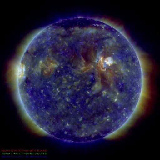
The Sun is doing it's thing as always. Not much too special to talk about today. For more data go to http://sdo.gsfc.nasa.gov/data/

 AIA 211 Angstrom band is red, AIA 193 Angstrom band is green, and AIA 171 is blue

In our back yard the robotic missions to Minor Planets Ceres and Pluto are really getting interesting.

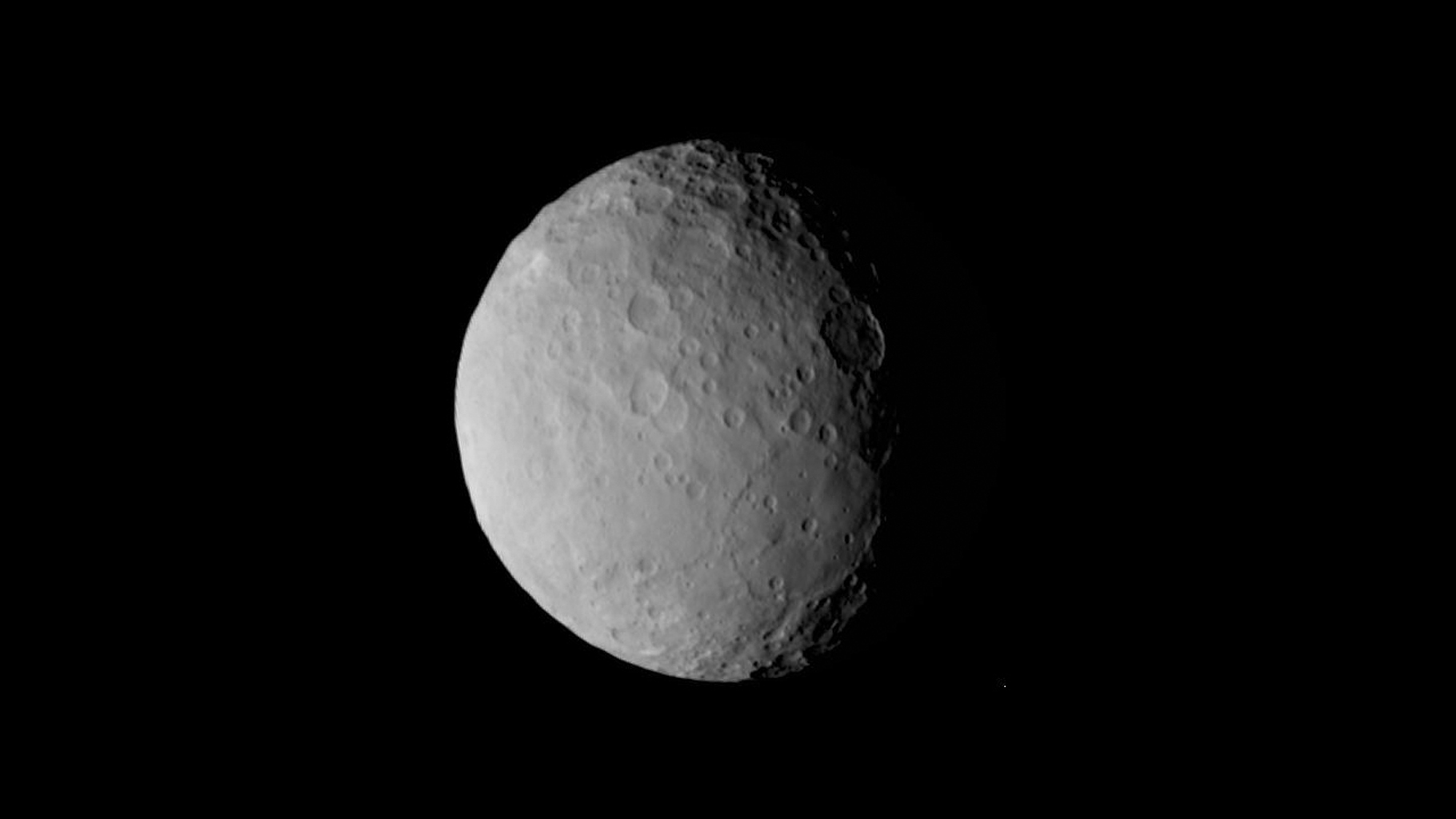
Dwarf planet Ceres as seen by NASA's DAWN mission

NASA's DAWN mission to Ceres is continuing its second mapping orbit. The CERES Image Of The Day website is worth looking at every now and again. The image on the right was taken on  Feb. 19, 2015 from a distance of nearly 29,000 miles (46,000 kilometers) from Ceres.

Fun Ceres facts: It is about 590 miles across, and accounts for about 25% of the entire asteroid belt's mass. Yet it is less than 1/14th of the mass of Plute, the other dwarf planet of note at the moment.

It is amazing to finally see non-deconvolved images of Pluto that actually look like something other than a blurry blob. [Read more at Space.com] Original images from JHU Applied Physics Lab.

New Horizon's image of Pluto and Charon taken on 06/29/2015 at a distance of 18 million km.

Sharpless 308. Copyright Kfir Simon

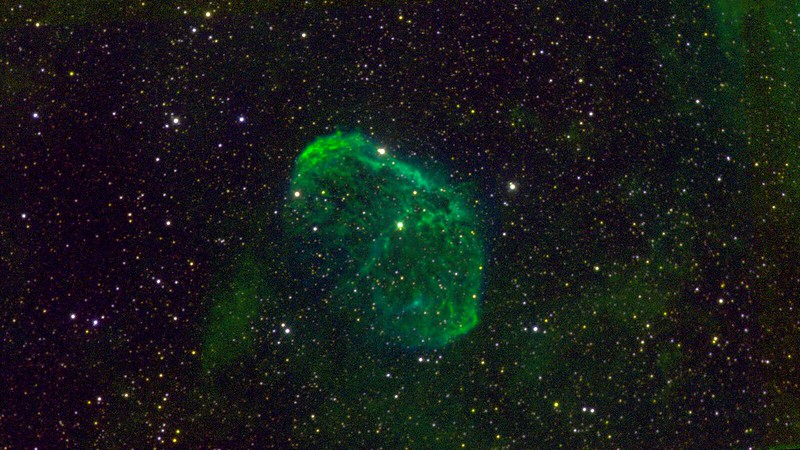
Bubbles. About 5,000 light years away from us is the beautiful Wolf-Rayet (stellar) bubble Sharpless 308. It is about 60 light years in diameter, and only 70,000 years old. The genetically modern human ancestors of ~98% or more of your DNA were present and still hanging out in Africa, but some were about to set off on extended holiday. [Credit: Kfir Simon, as seen on APOD]

Speaking of Wolf Rayet stars, how about Wolf Rayet galaxies? Why, it's a Hubble image of the famous SBS1415+437. (Just kidding, this galaxy is not well known, even among the so-called Wolf Rayet galaxies.)

The Wolf-Rayet galaxy SBS1415+437. Credit NASA/HST/Aloisi et al?

Go read the background at SpaceTelescope.org's Image of the Week. Although it is not clear from the Image of the Week site the image is probably that described in Aloisi et al, 2005, ApJ, 631, L45 which detected the presence of old (1+ Gyr) stars in SBS1415+437., which had bearing on an old (by now) debate about whether the so-called Wolf Rayet galaxies in the local Universe where young galaxies just experiencing their first burst of star formation (Answer: In general no, they're not).

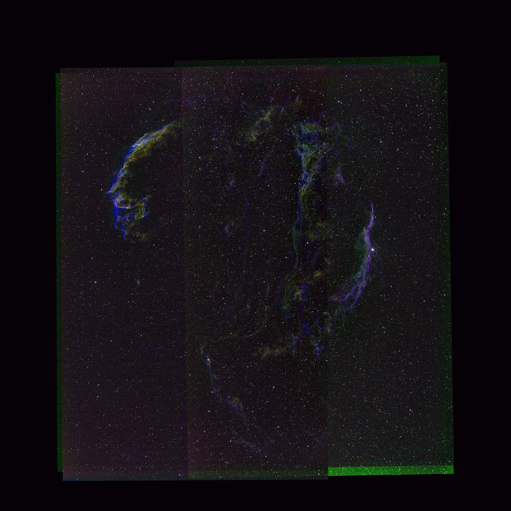
I of course chose the bubble, superbubble, Wolf Rayet galaxy, and NGC 6503 images because I did some work on wind-blown bubbles, superbubbles, WR galaxies and NGC 6503 back in the days I was a professional astronomer. Red and green Solar images are for Micah and Caelan, who are very into that type of solar imagery at the moment.

Exciting times in NGC 4666

I missed this when it happened in December, but a new Type Ia supernova was discovered in the "nearby" starburst galaxy NGC 4666 by the  Automated Sky Survey for SuperNovae (ASAS-SN) project on December 9th. Bob King at Universe Today has a nice short article with a finding chart for NGC 4666, and some background information and images of the galaxy. A more recent, early January, amateur observation showing the supernova by Justin Ng can be found at EarthSky.org.

More on this topic some time later...

High Energy Astronomy News

Two items of note:

1. Scientific American has a nice article on why the threat to life on Earth from Gamma Ray Bursts, in particular from the dying start Eta Carinae, is not something you need to worry about. (I've discussed putative GRB-caused events here and here).
2. NuSTAR, an orbitting hard X-ry telescope, has captured some cool images of hard X-ray emission from the Sun (not a target NuSTAR was expected to look at, being designed for the study of Active Galactic Nuclei millions to billions of light years from Earth).

The NuSTAR data, seen in green and blue, reveal solar high-energy emission (green shows energies between 2 and 3 kiloelectron volts, and blue shows energies between 3 and 5 kiloelectron volts). The high-energy X-rays come from gas heated to above 3 million degrees. The red channel represents ultraviolet light captured by SDO at wavelengths of 171 angstroms, and shows the presence of lower-temperature material in the solar atmosphere at 1 million degrees. [Image and caption from NASA/JPL]